Markov chain Monte Carlo
A different approach to sample distributions is based on the construction of a Markov chain.
It will turn out to be a very powerful approach.
It will also introduce some difficulties. In particular, the samples that will be generated are no longer going to be independent.
We will therefore have to be careful when estimating error bars.
Markov chain and transition probability
A Markov chain is a sequence of elements $x_1 \to x_2 \to x_3 \to x_4 \to \ldots$ generated by a Markov process.
It is characterized by a transition probability $p(x \to y)$. It is normalized $\sum_y p(x \to y) = 1$.
During the Markov process, a new element $x_{n+1}$ is added to the chain with a probability $p(x_n \to x_{n+1})$.
This transition probability only depends on the previous element, there is no memory of the distant past of the chain.
We will also suppose ergodicity, i.e. there is a non-zero probability path between any two $x$ and $y$.
Equilibrium probability distribution
What is the probability to be in a given $x$ at step $n+1$?
\begin{align*} \pi_{n+1} (x) &= \sum_{y \ne x} \pi_n(y) \, p(y \to x) + \pi_n(x) \, p(x \to x) \\ &= \sum_{y \ne x} \pi_n(y) \, p(y \to x) + \pi_n(x) \, \big( 1 - \sum_{y \ne x} p(x \to y) \big) \end{align*}
Suppose the distribution becomes stationary $\pi(x) = \pi_{n+1}(x) = \pi_n(x)$
Simplifying the equation above we obtain
\begin{equation*} \sum_{y \ne x} \pi(x) \, p(x \to y) = \sum_{y \ne x} \pi(y) \, p(y \to x) \end{equation*}
Global and detailed balance
Let's say we want to sample a distribution $\pi(x)$ using a Markov chain Monte Carlo.
It is enough to find a transition probability $p(x \to y)$ that satisfies the global balance condition
\begin{equation*} \boxed{ \sum_{y} \pi(x) \, p(x \to y) = \sum_{y} \pi(y) \, p(y \to x)} \end{equation*}
The condition above is necessary, but it is often simpler to design transition probabilities that satisfy the stronger detailed balance condition
\begin{equation*} \boxed{ \pi(x) \, p(x \to y) = \pi(y) \, p(y \to x)} \end{equation*}
The game is now to find a recipe to find $p(x \to y)$.
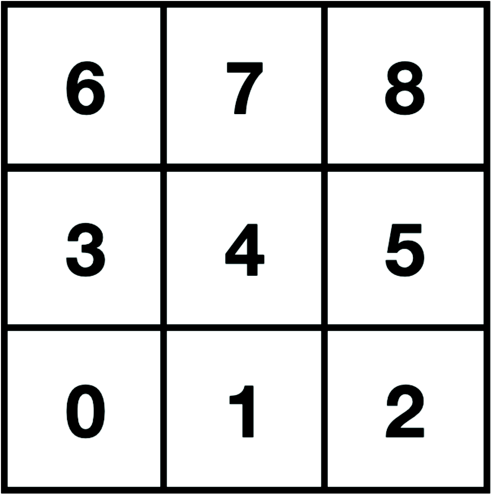
Example: the pebble game
Consider a $3 \times 3$ tiling. A pebble is sitting on one of the tiles $k \in \{0, \ldots, 8\}$.
We want to move the pebble to one of its neighbors with a transition probability $p(x \to y)$ such that the pebble will have a uniform distribution over the tiling $\pi_k = 1/9$.
The detailed balance imposes $p(x \to y) = p(y \to x)$.
We can use the following transition rules:
The probability to move to a neighbor is $1/4$. This ensures that $p(x \to y) = p(y \to x)$.
If there are less than 4 neighbors (edge, corner) the pebble can stay on its tile with the remaining probability.
L = 3
n_samples = 2**14
samples = np.zeros(n_samples, dtype=int)

for i in range(n_samples-1):

    # k -> (x,y)
    coord = np.unravel_index(samples[i], [L,L])

    # pick random shift (prob 1/4)
    ind = np.random.randint(2)
    shift = np.zeros(2, dtype=int)
    shift[ind] = np.random.choice([-1,1])

    # new (x,y) -> clip inside square -> k
    coord += shift
    samples[i+1] = np.ravel_multi_index(coord, [L,L], mode='clip')

Summary
Markov chain Monte Carlo (MCMC) is a different way to generate samples $x_i$ that are distributed according to some probability $\pi$.
A desired probability $\pi$ is obtained by choosing the transition probability such that it satifies the global balance condition
\begin{equation*} \sum_{y} \pi(x) \, p(x \to y) = \sum_{y} \pi(y) \, p(y \to x) \end{equation*}
or the detailed balance condition
\begin{equation*} \pi(x) \, p(x \to y) = \pi(y) \, p(y \to x) \end{equation*}
Finding a good transition probability is not trivial. If we change the rules of the pebble game and ask that the probability to sit on the tile $k$ is some $\pi_k$. What should I choose for $p(x \to y)$?
MCMC algorithms provide recipes to find $p(x \to y)$. There are many of them, e.g. the Glauber, Wolff, heat bath algorithms, etc. We will focus on the Metropolis-Hastings algorithm.
Unlike direct sampling, Markov chain sampling generates correlated samples. We will have to keep this in mind!