The two-dimensional Ising model
The Hamiltonian of the Ising model is
\begin{equation*} \mathcal{H} = -J \sum_{\langle i, j \rangle} \sigma_i \, \sigma_j \end{equation*}
where $\sigma_i = \pm 1$ is a spin living on the site $i$ of a periodic square lattice with $N = L \times L$ sites. We will consider a ferromagnetic coupling and set our unit of energy $J=1$.
We will be interested in computing the energy and the magnetization at a given temperature $T = 1/\beta$
\begin{equation*} \langle \mathcal{O} \rangle = \frac{1}{Z} \sum_{\sigma} e^{-\beta E(\sigma)} \, \mathcal{O}(\sigma) \qquad \text{where} \quad \mathcal{O} = E, m \end{equation*}
The sum is over all spin configurations $\sigma = \{\sigma_1, \ldots, \sigma_N\}$. This is a total of $2^N$ terms which quickly becomes intractable.
A Monte Carlo approach
We need to compute \begin{equation*} \langle \mathcal{O} \rangle = \frac{\sum_{\sigma} e^{-\beta E(\sigma)} \mathcal{O}(\sigma)} {\sum_{\sigma} e^{-\beta E(\sigma)}} \end{equation*}
It seems very natural to try to compute these integrals using the Boltzmann probability
\begin{equation*} \pi(\sigma) = \frac{e^{-\beta E(\sigma)}}{Z} \quad \to \quad \langle \mathcal{O} \rangle = \frac{\sum_{\sigma} \pi(\sigma) \, \mathcal{O}(\sigma) Z} {\sum_{\sigma} \pi(\sigma) \, Z} = \frac{\sum_{\sigma} \pi(\sigma) \, \mathcal{O}(\sigma)} {\sum_{\sigma} \pi(\sigma)} \simeq \frac{\sum_\sigma^\mathrm{MC} \mathcal{O}(\sigma)}{\sum_\sigma^\mathrm{MC} 1} \end{equation*}
We got lucky: we do not know how to normalize the Boltzmann probability. But this normalization constant cancels in the fraction.
$\sum^\mathrm{MC}_\sigma$ means a sum over samples $\sigma$ distributed according to $\pi(\sigma)$. Because the distribution is the same in the numerator and denominator, we can compute both sums from the same samples.
We can use Metropolis-Hastings to sample $\pi(\sigma)$.
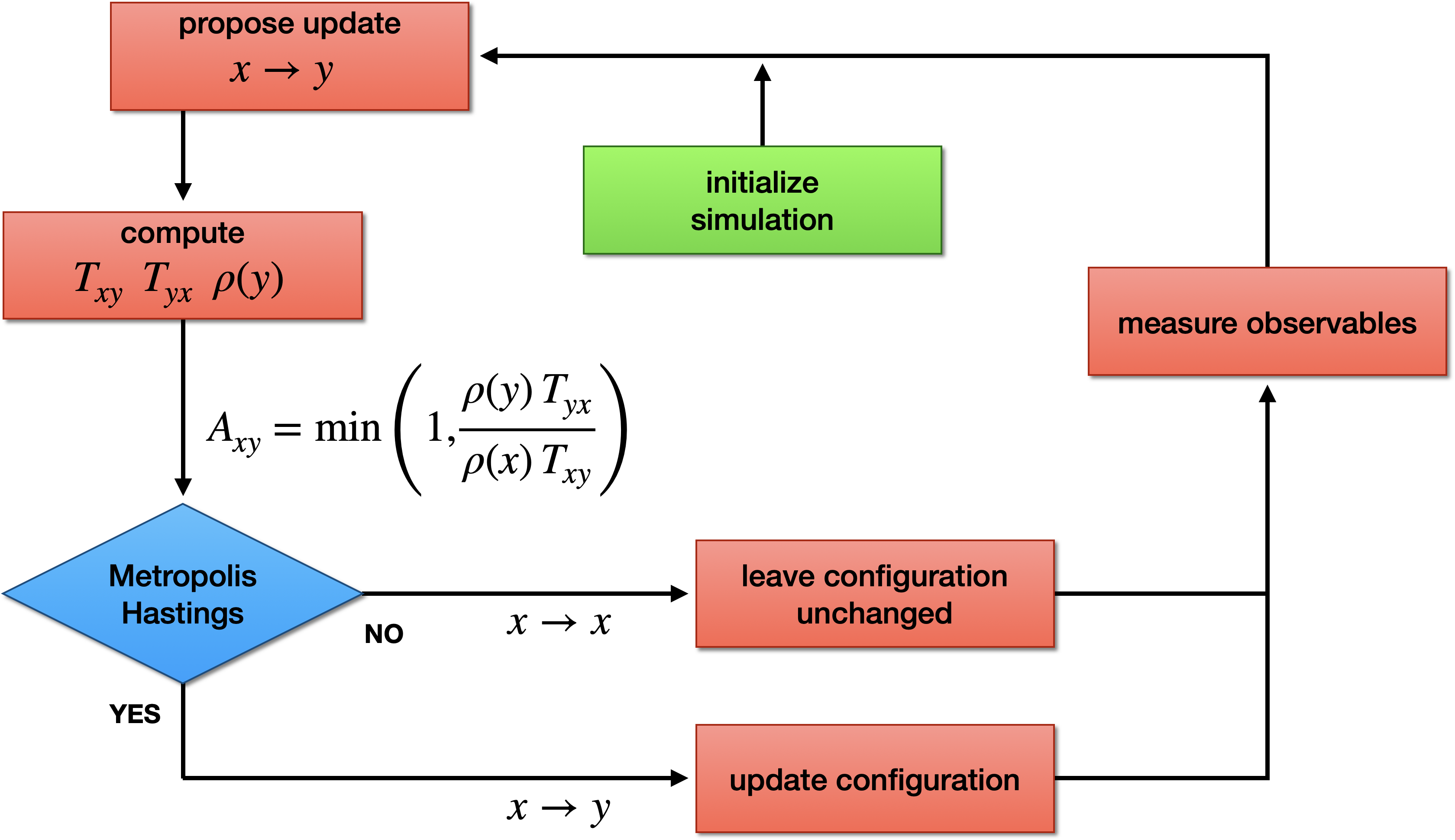
Metropolis-Hastings algorithm
We have to choose our proposal probability $T(\sigma \to \sigma')$.
A possible choice is to pick a random site $i$ and flip $\sigma_i$
\begin{equation*} T(\sigma \to \sigma') = \begin{cases} 1/N & \text{if $\sigma$ and $\sigma'$ differ by a single spin flip} \\ 0 & \text{otherwise} \end{cases} \end{equation*}
Acceptance probability
\begin{equation*} A(\sigma \to \sigma') = \min \left( 1, \frac{\pi(\sigma')}{\pi(\sigma)} \right) = \min \left( 1, \frac{e^{-\beta E(\sigma')}}{e^{-\beta E(\sigma)}} \right) = \min \left( 1, e^{-\beta \Delta E} \right) \end{equation*}
Again only a ratio of $\pi$'s appears and $Z$ cancels out.
We only need to compute $\Delta E$. Because the change is local, this calculation is quick.
def initialize(L):
    σ = np.random.choice([-1,1], size=(L,L))
    return σ

def monte_carlo_step(σ, β):

    L = σ.shape[0]

    # try L^2 flips
    for i in range(L**2):

        k, l = np.random.randint(L, size=2) # pick a site
        ΔE = 2 * σ[k,l] * (σ[(k+1)%L,l] + σ[(k-1)%L,l] + σ[k,(l+1)%L] + σ[k,(l-1)%L])

        # accept the flip
        if np.random.rand() < np.exp(-β * ΔE):
            σ[k,l] *= -1

    return σ
fig, ax = plt.subplots(2, 5, figsize=(8,4))
for i, β in enumerate([0.1, 1.5]):

    σ = initialize(32)
    for j in range(5):

        ax[i,j].matshow(σ)
        ax[i,j].set_xticks([]);
        ax[i,j].set_yticks([]);
        if i==1: ax[i,j].text(14, 36, f"step = {j*5}", fontsize=10)
        if j==4: ax[i,j].text(36, 16, fr'$\beta = {β}$')

        for k in range(5):
            monte_carlo_step(σ, β)

fig.tight_layout(h_pad=-2.5, w_pad=0.5)

Computing observables
- We can compute the energy and the magnetization
def compute_energy(σ):
    L = σ.shape[0]
    E = 0
    for k in range(L):
        for l in range(L):
            E -= σ[k,l] * (σ[(k+1)%L,l] + σ[k,(l+1)%L])
    return E / L**2

def compute_magnetization(σ):
    L = σ.shape[0]
    return np.sum(σ) / L**2
# A single Monte Carlo run
n_samples = 2**10
energies = np.zeros(n_samples)
magnetizations = np.zeros(n_samples)

L = 8
T = 2.0
β = 1 / T
σ = initialize(L)

# MC simulation
for k in range(n_samples):

    monte_carlo_step(σ, β)
    energies[k] = compute_energy(σ)
    magnetizations[k] = compute_magnetization(σ)

# Compute several temperatures
Tr = np.linspace(1, 3, 10)[::-1]
n_T = Tr.size
L = 8
σ = initialize(L)

n_samples = 2**11
n_warmup = 200
energies = np.zeros([n_samples, n_T])
magnetizations = np.zeros([n_samples, n_T])

for i, T in enumerate(Tr):

    β = 1 / T
    for k in range(n_samples + n_warmup):

        # MC moves
        monte_carlo_step(σ, β)

        # measure after thermalization
        if k >= n_warmup:
            energies[k-n_warmup, i] = compute_energy(σ)
            magnetizations[k-n_warmup, i] = compute_magnetization(σ)

fig, ax = plt.subplots()

m = np.average(magnetizations, axis=0)
σₘ = np.std(magnetizations, axis=0) / np.sqrt(n_samples) # Danger!

ax.errorbar(Tr, np.abs(m), yerr=σₘ, marker='x', markersize=4, label=f"MC ${L} \\times {L}$")
ax.axvline(2.0/np.log(1.0+np.sqrt(2.0)), color='gray', linestyle='--', label="Onsager")
ax.set_title("Magnetization")
ax.set_xlabel("$T$")
ax.set_ylabel("$m$")
ax.grid(alpha=0.2)
ax.legend();

Summary
We have successfully used the Metropolis-Hastings algorithm to simulate the two-dimensional Ising model.
The local update of a spin is fast but generates long correlation length.
This leads to wrong estimates of the error bars with the naive formula.
We will see how to compute error bars and good estimators.
Note that there are many other efficient MCMC algorithms for the Ising model, e.g. cluster algorithms.